Showcase

library(here)
source(here("setup.R"))
options(encoding = "UTF-8")
Sys.setlocale("LC_ALL", "C")

here() starts at /Users/stefan/workspace/work/phd/thesis

'C/C/C/C/C/de_DE'

full_truth_county <- read_csv(here("data/processed/RKI_county_weekly.csv")) %>%
    arrange(date, ags)

full_truth <- full_truth_county %>%
    group_by(date) %>%
    summarize(cases = sum(cases, na.rm = TRUE))

ags_county_dict <- read_csv(here("data/processed/ags_county_dict.csv")) %>%
    arrange(ags) %>%
    mutate(c = 1:n())

population <- read_csv(here('data/processed/population.csv'))

showcase_results <- read_csv(here("data/results/4_local_outbreak_model/showcase.csv"))

y_total_result <- showcase_results %>% 
    filter(variable == "y_total")

rename_pct_to_decimal <- function(x) as.numeric(gsub("%", "", x)) / 100

y_total_dist <- y_total_result %>% 
    select(ends_with('%')) %>%
    pivot_longer(cols = everything(), names_to = "percentile", values_to = "value") %>%
    mutate(percentile = rename_pct_to_decimal(percentile)) %>%
    bind_rows(tibble(value = c(0, Inf), percentile = c(0, 1))) %>%
    arrange(value)

Comparison to NBinom baseline

prediction_date <- showcase_results %>% pull(date) %>% max
baseline_df <- full_truth %>%
    filter(date <= prediction_date - 7, date >= prediction_date - 14) 

growth_rate <- baseline_df %>%
    pull(cases) %>%
    log %>% diff %>% exp


lambda_old <- baseline_df %>%
    pull(cases) %>%
    tail(1)

lambda_new <- lambda_old * growth_rate

growth_rate
lambda_old
lambda_new

1.66609294320138

3872

6451.11187607574

baseline_county <- full_truth_county %>% filter(date <= prediction_date - 7, date >= prediction_date - 14)
I_old_county <- baseline_county %>%
    group_by(ags) %>%
    summarize(cases = cases[2]) 

emp_rho_c <- baseline_county %>%
    group_by(ags) %>%
    summarize(growth_rate = exp(diff(log(cases)))) 
rho_c_cleaned <- emp_rho_c %>%
    mutate(growth_rate = ifelse(is.na(growth_rate) | is.infinite(growth_rate), 1.0, growth_rate)) %>%
    mutate(growth_rate = pmin(growth_rate, 3))

lambda_new_county <-  rho_c_cleaned %>%
    inner_join(I_old_county) %>%
    mutate(intensity_prediction = growth_rate * cases) %>%
    pull(intensity_prediction)

Joining with `by = join_by(ags)`

total_nb_obs <- full_truth %>%
    filter(date >= ymd('2020-04-25'), date<= prediction_date - 7) %>%
    mutate(rho = cases / lag(cases)) %>%
    mutate(predicted = lag(cases) * lag(rho)) %>%
    tail(-2) %>%
    dplyr::select(y = cases, mu = predicted)

est_r <- function(df) {
    loglik <- function(r) -sum(dnbinom(df$y, mu = df$mu, size = r))
    r_est <- optimize(loglik, interval=c(1e-3,1e3))$minimum
}

r_country <- est_r(total_nb_obs)
nb_quantiles <- qnbinom(y_total_dist$percentile, mu = lambda_new, size = r_country) %>%
    tibble(
        percentile = y_total_dist$percentile,
        value = .
    ) %>%
    pivot_wider(names_from = percentile, values_from = value) %>%
    mutate(date = prediction_date)
nb_quantiles

r_country

A tibble: 1 × 26

0	0.01	0.025	0.05	0.1	0.15	0.2	0.25	0.3	0.35	⋯	0.7	0.75	0.8	0.85	0.9	0.95	0.975	0.99	1	date
<dbl>	<dbl>	<dbl>	<dbl>	<dbl>	<dbl>	<dbl>	<dbl>	<dbl>	<dbl>	⋯	<dbl>	<dbl>	<dbl>	<dbl>	<dbl>	<dbl>	<dbl>	<dbl>	<dbl>	<date>
0	5250	5426	5581	5763	5888	5988	6076	6155	6228	⋯	6726	6810	6905	7017	7159	7373	7562	7786	Inf	2020-06-27

143.094444769947

lambda_new_county[99]

2568

N_samples <- 1e5
total_county_nb_obs <- full_truth_county %>%
    filter(date >= ymd('2020-04-25'), date<= prediction_date - 7) %>%
    group_by(ags) %>%
    mutate(rho = cases / lag(pmax(cases, 1))) %>%
    mutate(predicted = pmax(lag(cases) * lag(rho), 1)) %>%
    ungroup() %>%
    filter(!is.na(predicted)) %>%
    dplyr::select(ags, y = cases, mu = predicted)

county_rs <- total_county_nb_obs %>%
    group_by(ags) %>%
    summarize(r = est_r(cur_data())) %>%
    mutate(mu = lambda_new_county)

nbinom_county_samples <- rnbinom(N_samples * 400, mu = county_rs$mu, size = county_rs$r) %>%
    matrix(c(400, N_samples)) 

nb_county_quantiles <-  nbinom_county_samples %>%
    pmin(population$population) %>%
    colSums %>%
    quantile(probs = y_total_dist$percentile) %>%
    tibble(
        percentile = y_total_dist$percentile,
        value = .
    ) %>%
    pivot_wider(names_from = percentile, values_from = value) %>%
    mutate(date = prediction_date)
nb_county_quantiles_no_GL <- nbinom_county_samples[-99,] %>%
    colSums %>%
    quantile(probs = y_total_dist$percentile) %>%
    tibble(
        percentile = y_total_dist$percentile,
        value = .
    ) %>%
    pivot_wider(names_from = percentile, values_from = value) %>%
    mutate(date = prediction_date)

Warning message:

"There was 1 warning in `summarize()`.

i In argument: `r = est_r(cur_data())`.

i In group 1: `ags = "01001"`.

Caused by warning:

! `cur_data()` was deprecated in dplyr 1.1.0.

i Please use `pick()` instead."

nb_county_quantiles

A tibble: 1 × 26

0	0.01	0.025	0.05	0.1	0.15	0.2	0.25	0.3	0.35	⋯	0.7	0.75	0.8	0.85	0.9	0.95	0.975	0.99	1	date
<dbl>	<dbl>	<dbl>	<dbl>	<dbl>	<dbl>	<dbl>	<dbl>	<dbl>	<dbl>	⋯	<dbl>	<dbl>	<dbl>	<dbl>	<dbl>	<dbl>	<dbl>	<dbl>	<dbl>	<date>
4759	5611.99	5829	6035	6282	6465	6619	6759	6888	7011	⋯	7957	8139	8358	8631	9018	9778	11061.02	16065.13	249228	2020-06-27

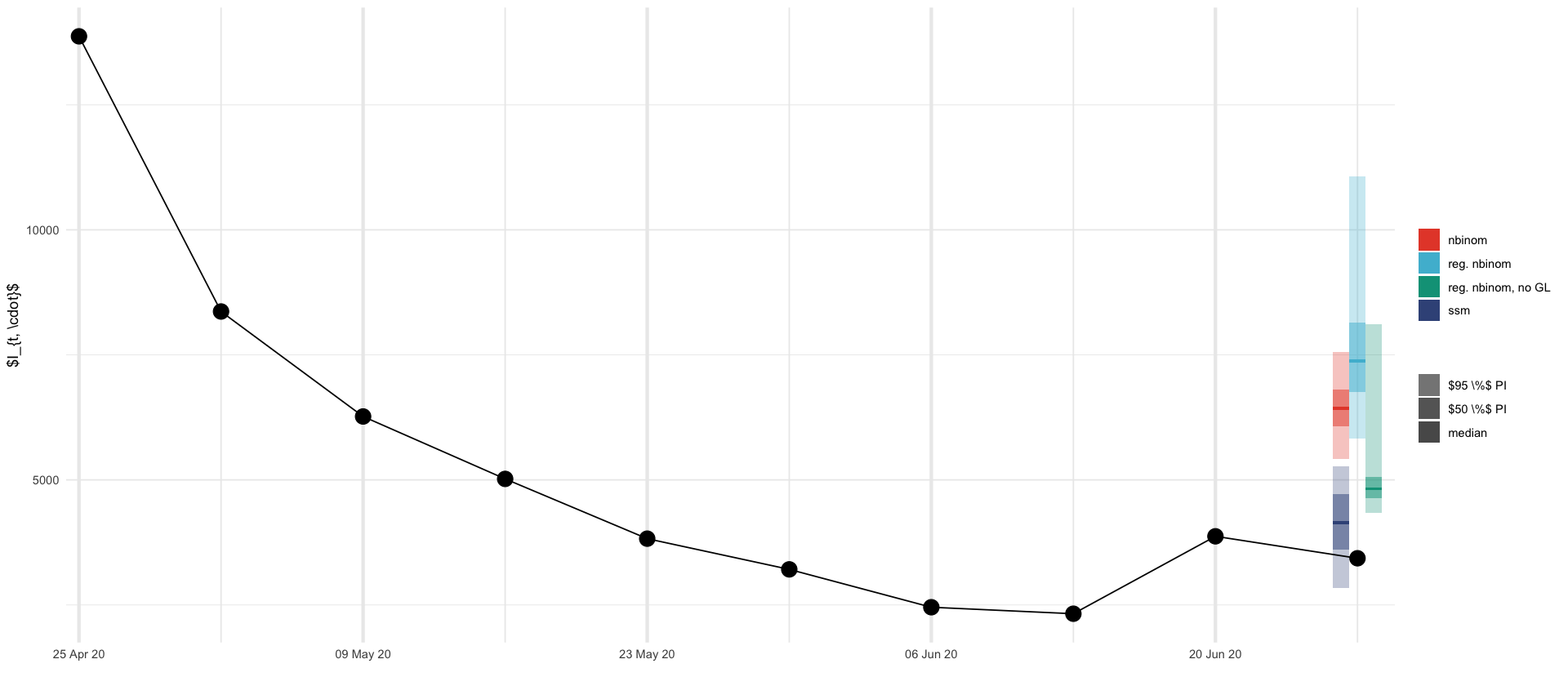
tikz/regional_showcase_predictions.tex

y_total_result

A spec_tbl_df: 1 × 29

variable	c	t	mean	sd	1.0 %	2.5 %	5.0 %	10.0 %	15.0 %	⋯	65.0 %	70.0 %	75.0 %	80.0 %	85.0 %	90.0 %	95.0 %	97.5 %	99.0 %	date
<chr>	<dbl>	<dbl>	<dbl>	<dbl>	<dbl>	<dbl>	<dbl>	<dbl>	<dbl>	⋯	<dbl>	<dbl>	<dbl>	<dbl>	<dbl>	<dbl>	<dbl>	<dbl>	<dbl>	<date>
y_total	0	10	4170.382	666.6667	2261.53	2842.372	3605.151	3605.479	3605.806	⋯	4721.306	4721.794	4722.282	4722.769	4723.257	4723.745	5012.9	5277.69	5281.091	2020-06-27

dx <- .4

alpha_fct <- factor(c("median", "$50 \\%$ PI", "$95 \\%$ PI"), levels=c("median", "$50 \\%$ PI", "$95 \\%$ PI"))
col = pal_npg("nrc")(10)[3]


geom_prediction_interval <- function(model, data, dx=1, offset=0) {
    list(
        geom_rect(aes(xmin = date - dx + offset, xmax= date+dx + offset, ymin = `0.025`, ymax = `0.975`, alpha=alpha_fct[3], fill=model), data=data),
        geom_rect(aes(xmin = date - dx + offset, xmax= date+dx + offset, ymin = `0.25`, ymax = `0.75`, alpha=alpha_fct[2], fill=model), data=data),
        geom_rect(aes(xmin= date - dx + offset, xmax=date + dx + offset, ymin = `0.5`-30, ymax=`0.5`+30, alpha=alpha_fct[1], fill=model), data=data)
    )
}

y_result_plot <- y_total_result %>%
    rename_with(function(x) as.character(rename_pct_to_decimal(x)), ends_with('%')) 

full_truth %>%
    inner_join(y_result_plot, by=c("date"="date")) %>%
    ggplot(aes()) +
    geom_prediction_interval("ssm", data=y_result_plot, dx=dx, offset=-2*dx) +
    geom_prediction_interval("nbinom", data=nb_quantiles, dx=dx,offset=-2*dx) +
    geom_prediction_interval("reg. nbinom", data=nb_county_quantiles, dx=dx, offset=0*dx) +
    geom_prediction_interval("reg. nbinom, no GL", data=nb_county_quantiles_no_GL, dx=dx, offset=2*dx) +

    geom_line(aes(date, cases), data= full_truth %>% filter(date >= ymd('2020-04-25'), date <= ymd('2020-06-27'))) +
    geom_point(aes(date, cases), data= full_truth %>% filter(date >= ymd('2020-04-25'), date <= ymd('2020-06-27')), size=5)  +
    scale_alpha_manual(name="", values=c("median"=1, "$50 \\%$ PI"=0.5, "$95 \\%$ PI"=0.3)) +
    labs(x="", y="$I_{t, \\cdot}$", fill="") +
    scale_x_date(
        breaks = function(x) seq(ceiling_date(x[1], "week", week_start = 6), floor_date(x[2], "week", week_start = 6), by = "2 week"),
        date_labels = "%d %b %y",
        expand = expansion(mult = c(0.01, 0.01))
    ) +
    theme(
        panel.grid.major.x = element_line(linewidth = 1.2),
        panel.grid.minor.x = element_line(linewidth = 0.5)
    ) +
    scale_fill_npg()

ggsave_tikz(here("tikz/regional_showcase_prediction.tex"), width=16/1.5, height=7/1.5)

pdf: 2

full_truth %>%
    filter(date <= prediction_date, date >= prediction_date - 21)

A tibble: 4 × 2

date	cases
<date>	<dbl>
2020-06-06	2454
2020-06-13	2324
2020-06-20	3872
2020-06-27	3433

tables/regional_showcase_theta.tex

parameters <- read_csv(here("data/results/4_local_outbreak_model/estimated_parameters.csv"), col_names = c("parameter", "value")) %>% 
    pivot_wider(names_from = parameter, values_from = value) %>%
    rename(
        "$\\alpha$" = alpha,
        "$\\sigma_{\\overline{\\log \\rho}}$" = sigma_r,
        "$\\sigma_{S}$" = "sigma spatial",
        "$\\bar{q}$" = q,
        "$C$" = C,
        "$r$" = r
    ) %>%
    pivot_longer(everything(), names_to="parameter", values_to="estimate")

parameters %>%
    kable(format = "latex", digits=3, booktabs=T, escape=F) %>%
    cat(., file=here("tables/regional_showcase_theta.tex"))

log_rhos <- showcase_results %>%
    filter(str_starts(variable, "log_rho_")) %>%
    # extract both indices from variable names like log_rho_2_1
    mutate(c = as.numeric(str_extract(variable, "log_rho_(\\d+)_(\\d+)", group=1))) %>%
    mutate(t = as.numeric(str_extract(variable, "log_rho_(\\d+)_(\\d+)", group=2))) 
log_rhos %>%
    head()

log_rhos %>%
    mutate(c = factor(c)) %>%
    ggplot(aes(t, exp(mean), group=c)) +
    geom_line(show.legend=FALSE, alpha=1/100) +
    xlim(NA, 9) +
    scale_y_log10()

A tibble: 6 × 29

variable	c	t	mean	sd	1.0 %	2.5 %	5.0 %	10.0 %	15.0 %	⋯	65.0 %	70.0 %	75.0 %	80.0 %	85.0 %	90.0 %	95.0 %	97.5 %	99.0 %	date
<chr>	<dbl>	<dbl>	<dbl>	<dbl>	<dbl>	<dbl>	<dbl>	<dbl>	<dbl>	⋯	<dbl>	<dbl>	<dbl>	<dbl>	<dbl>	<dbl>	<dbl>	<dbl>	<dbl>	<date>
log_rho_1_1	1	1	-1.2163769	0.1598178	-1.68070449	-1.38564169	-1.38209844	-1.23059352	-1.2302142	⋯	-1.2264477	-1.2263806	-1.2263136	-1.2262465	-1.2261794	-1.2261123	-0.9170889	-0.6766719	-0.6762008	2020-04-25
log_rho_2_1	2	1	0.5549448	0.2022438	0.01482255	0.01658301	0.01830238	0.07906171	0.6228041	⋯	0.6312126	0.6315221	0.6318316	0.6321411	0.6324505	0.6327600	0.6330695	0.6332242	0.6333171	2020-04-25
log_rho_3_1	3	1	-1.2193435	0.1411181	-1.73760412	-1.73510571	-1.73333119	-1.39045531	-1.1816277	⋯	-1.1714910	-1.1714093	-1.1713275	-1.1712457	-1.1711639	-1.1710822	-1.1710004	-1.1709595	-1.1709350	2020-04-25
log_rho_4_1	4	1	0.3627378	0.1114700	-0.40008267	0.28558075	0.28945849	0.37452239	0.3799041	⋯	0.3847352	0.3848608	0.3849863	0.3851119	0.3852374	0.3853630	0.3854885	0.3855513	0.3855889	2020-04-25
log_rho_5_1	5	1	-1.6572183	0.5181756	-3.50727209	-3.49655451	-3.47869189	-2.22266098	-1.5013308	⋯	-1.4963833	-1.4962190	-1.4960547	-1.4958903	-1.4957260	-1.4955616	-1.4953973	-1.4953151	-0.9410035	2020-04-25
log_rho_6_1	6	1	-0.2124819	0.1065888	-0.54829519	-0.54787938	-0.54719614	-0.36253192	-0.1835588	⋯	-0.1812240	-0.1811594	-0.1810947	-0.1810301	-0.1809654	-0.1809007	-0.1808361	-0.1808037	-0.1807844	2020-04-25

Warning message:

"Removed 400 rows containing missing values or values outside the scale range

(`geom_line()`)."

approaches <- factor(c("ssm", "empirical"), levels = c("ssm", "empirical"))

ssm_app <- approaches[1]
empirical_app <- approaches[2]

emp_rho_plt <- full_truth_county %>%
    filter(date >= ymd('2020-04-18'), date<= prediction_date - 7) %>%
    group_by(ags) %>% 
    mutate(rho = cases / lag(pmax(cases, 1))) %>%
    filter(!is.na(rho)) 

showcase_results %>%
    filter(variable == "log_rho") %>%
    ggplot(aes(date, exp(`50.0 %`), color=ssm_app)) +
    geom_boxplot(aes(date-1, rho, color=empirical_app, group = date, linetype='county'), data = emp_rho_plt, width=2) +
    geom_boxplot(aes(date+1, group = date, color=ssm_app, linetype='county'), data = log_rhos, width=2) +
    geom_line(aes(linetype='country'), linewidth=2) +
    geom_line(data = full_truth %>% mutate(rho = cases / lag(cases)), aes(date, rho, color=empirical_app, linetype='country'), linewidth=2) +
    ylim(0,4) +
    scale_x_date(
        breaks = function(x) seq(ceiling_date(x[1], "week", week_start = 6), floor_date(x[2], "week", week_start = 6), by = "2 week"),
        date_labels = "%d %b %y",
        expand = expansion(mult = c(0.01, 0.01)),
        limits = c(ymd('2020-04-20'), ymd('2020-06-24'))
    ) +
    labs(color="approach", linetype='level', x="", y="$\\rho_{t}$") +
    scale_linetype_manual(values = c('county'='solid', 'country'='dashed')) 

ggsave_tikz(here("tikz/regional_showcase_rho.tex"), width=16/1.5, height=7/1.5)

Warning message:

"Removed 97 rows containing non-finite outside the scale range

(`stat_boxplot()`)."

Warning message:

"Removed 400 rows containing missing values or values outside the scale range

(`stat_boxplot()`)."

Warning message:

"Removed 49 rows containing non-finite outside the scale range

(`stat_boxplot()`)."

Warning message:

"Removed 1 row containing missing values or values outside the scale range

(`geom_line()`)."

Warning message:

"Removed 166 rows containing missing values or values outside the scale range

(`geom_line()`)."

Warning message:

"Removed 97 rows containing non-finite outside the scale range

(`stat_boxplot()`)."

Warning message:

"Removed 400 rows containing missing values or values outside the scale range

(`stat_boxplot()`)."

Warning message:

"Removed 49 rows containing non-finite outside the scale range

(`stat_boxplot()`)."

Warning message:

"Removed 1 row containing missing values or values outside the scale range

(`geom_line()`)."

Warning message:

"Removed 166 rows containing missing values or values outside the scale range

(`geom_line()`)."

pdf: 2

log_rhos %>% 
    filter(date == prediction_date - 7) %>%
    inner_join(full_truth_county %>% filter(date == prediction_date - 7) %>% mutate(c = 1:400) %>% select(c, cases)) %>%
    select(`50.0 %`, cases)  %>%
    mutate(mu = exp(`50.0 %`) * cases)  %>%
    filter(cases > 19)

Joining with `by = join_by(c)`

A tibble: 32 × 3

50.0 %	cases	mu
<dbl>	<dbl>	<dbl>
0.22141410	27	33.69168
0.13619816	27	30.93954
0.81227614	135	304.15910
0.16651360	77	90.95083
-0.19824822	28	22.96465
-0.46848131	43	26.91594
0.42210002	96	146.41546
0.21066202	82	101.22859
0.26134013	28	36.36274
0.51631338	23	38.54428
1.30123256	29	106.54084
-0.37364730	24	16.51727
0.09001093	38	41.57908
0.82648694	24	54.84663
0.56741722	31	54.67488
2.46741720	193	2275.84658
2.48864543	856	10310.47665
0.38797962	54	79.59599
1.17074579	26	83.83431
1.32054362	29	108.61825
0.88694198	37	89.82469
-0.04494725	52	49.71449
1.00240337	31	84.46950
0.62712586	23	43.06110
0.02060513	27	27.56211
-0.56278372	22	12.53167
0.90301542	21	51.80765
0.26862714	57	74.56554
0.17735707	22	26.26926
0.74328202	536	1127.11458
3.21901521	27	675.09409
0.96394301	84	220.24924

log_rhos %>% 
    filter(date == prediction_date - 7) %>%
    ggplot(aes(exp(`50.0 %`))) +
    geom_histogram()

`stat_bin()` using `bins = 30`. Pick better value with `binwidth`.

showcase_results %>%
    filter(str_starts(variable, "y_total_")) %>%
    mutate(c = as.numeric(str_extract(variable, "y_total_(\\d+)", group=1))) %>%
    inner_join(mutate(ags_county_dict, c=1:400), by = "c") %>%
    inner_join(filter(full_truth_county, date == '2020-06-13'), by=c("ags")) %>%
    filter(mean >= 100) %>%
    arrange(desc(mean)) %>%
    ggplot(aes(y = name, x = mean)) +
    geom_errorbarh(aes(xmin = `2.5 %`, xmax = `97.5 %`)) +
    geom_point(aes(x = `50.0 %`), pch='x', color='red', size=10) +
    geom_point(aes(x = cases))

Exchange matrix P

ags_county_dict <- read_csv(here("data/processed/ags_county_dict.csv"))
ags_state_dict <- read_csv(here("data/processed/ags_state_dict.csv"))

index_to_state <- ags_county_dict %>% 
    mutate(i = 1:400) %>%
    mutate(state_ags = str_sub(ags, end=2)) %>%
    rename(county_name = name) %>%
    inner_join(ags_state_dict, by=c("state_ags"="ags"))  %>%
    select(i, state_ags, county_name, state_name = name)

P <- read_delim(here("data/results/4_local_outbreak_model/showcase_P_matrix.csv"), delim = " ", col_names = 1:400) %>%
    as.matrix()


colnames(P) <- NULL
P_long_states <- melt(P) %>%
    rename(i = Var1, j = Var2) %>%
    inner_join(select(index_to_state, i, state_name_i = state_name), by=c("i")) %>%
    inner_join(select(index_to_state, j=i, state_name_j = state_name), by=c("j")) 
    
P_long_states %>%
    filter(state_name_i == state_name_j) %>%
    ggplot(aes(i,-j, fill=value)) +
    geom_tile() +
    scale_fill_gradient2(
        low = "white",
        mid = pal_npg("nrc")(5)[5],
        high = pal_npg("nrc")(5)[1],
        midpoint = 0.55,  # Set midpoint where you want emphasis
        limits = c(0,1)
    ) +
    facet_wrap(~state_name_i, scales="free") +
    theme_void() +
    labs(fill= "$p_{r,r'}$")


ggsave_tikz(here("tikz/P_matrix.tex"))

pdf: 2

tibble(
    total = colSums(P),
    i = 1:400,
    p_ii = diag(P)
) %>%
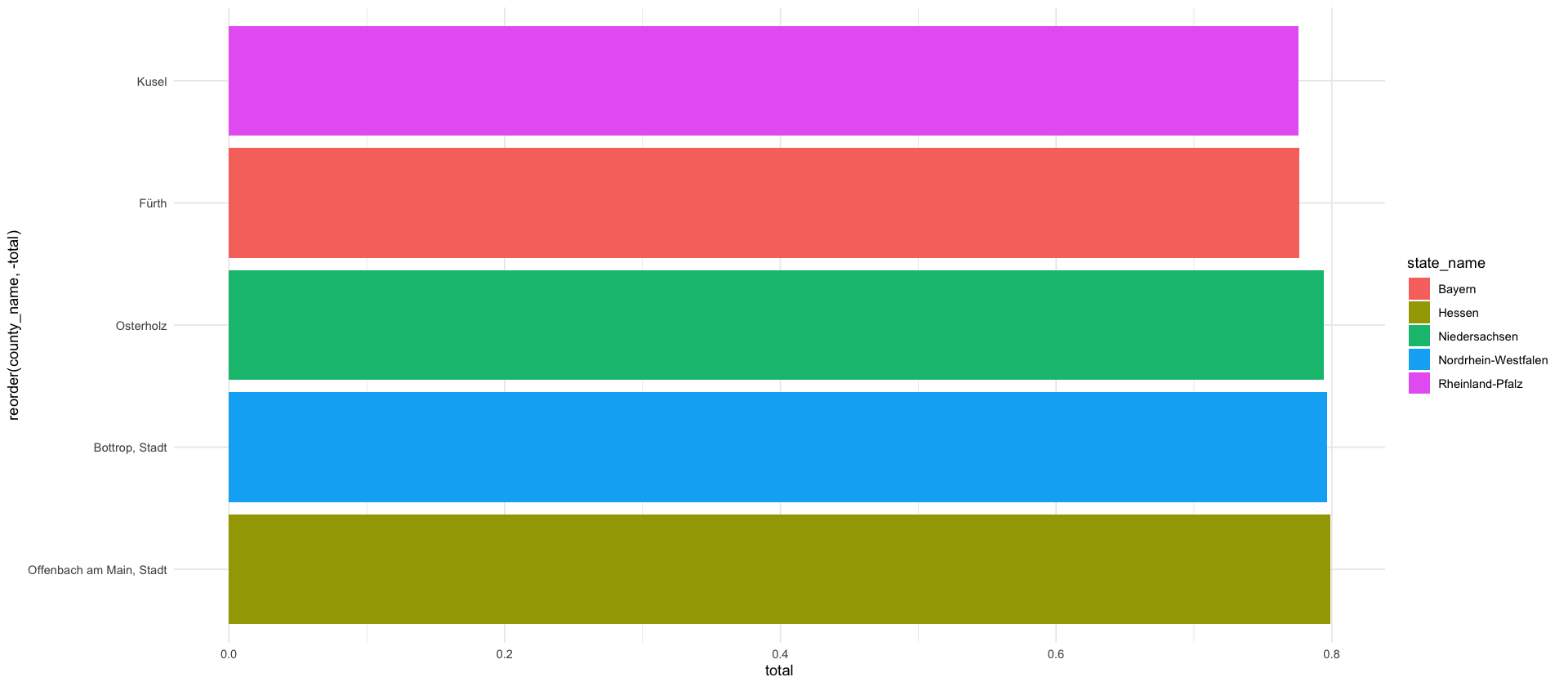
    inner_join(index_to_state, by=c("i")) %>%
    filter(total < 0.8) %>%
    ggplot(aes(x = reorder(county_name, -total), y = total, fill=state_name)) +
    geom_bar(stat = "identity") +
    coord_flip()

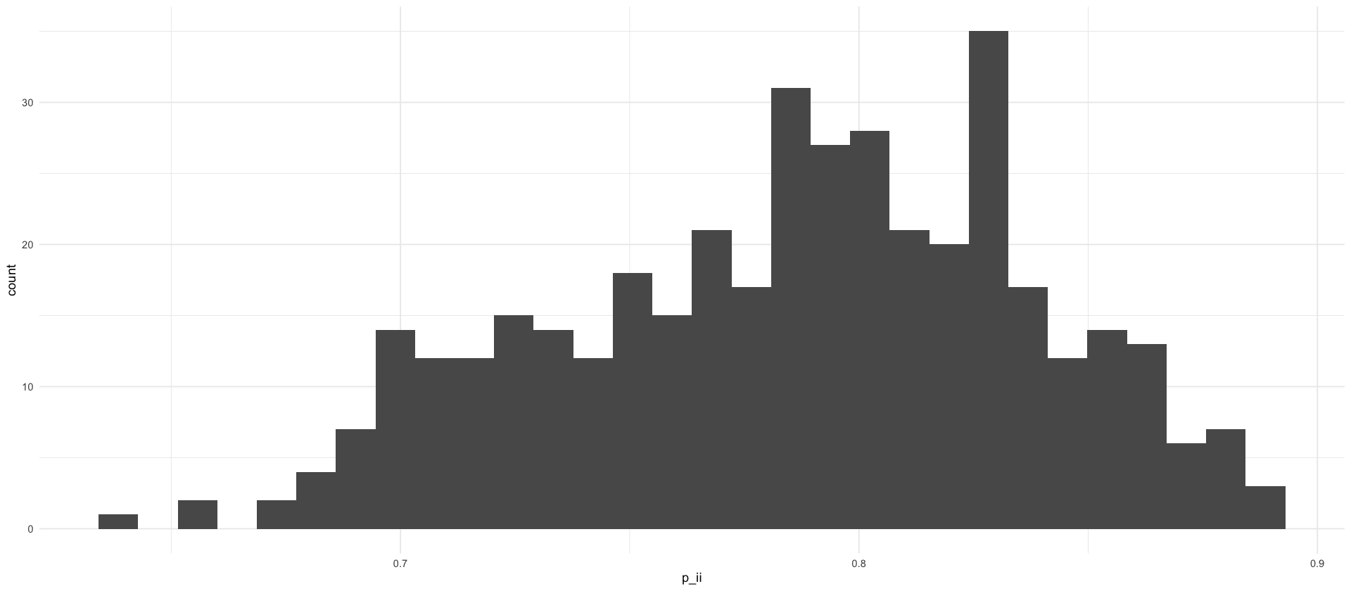
tibble(
    p_ii = diag(P),
    i = 1:400
) %>%
    inner_join(index_to_state, by=c("i")) %>%
    ggplot(aes(x = p_ii)) +
    geom_histogram()

`stat_bin()` using `bins = 30`. Pick better value with `binwidth`.

# solve utf-8 encoding issues
Sys.setlocale("LC_ALL", "UTF-8")

'C/UTF-8/C/C/C/de_DE'

county_shorthand <- function(county_name) {
    ifelse(
        str_detect(county_name, "Stadt"),
        paste0(str_sub(county_name, 1, 3), ". Stadt"),
        paste0(str_sub(county_name, 1, 3), ".")
    )
}

saxony_ags <- ags_state_dict %>%
    filter(name == "Sachsen") %>%
    pull(ags)

saxony_counties <- ags_county_dict %>%
    mutate(i = 1:400) %>%
    filter(str_starts(ags, saxony_ags)) %>%
    rename(county_name = name) %>%
    select(i, county_name)


P_saxony <- melt(P) %>%
    rename(i = Var1, j = Var2) %>%
    inner_join(select(saxony_counties, i, county_name_i = county_name), by=c("i")) %>%
    inner_join(select(saxony_counties, j=i, county_name_j = county_name), by=c("j"))  



p_rr <- P_saxony %>%
    filter(i == j) %>%
    mutate(county_name_i_short = county_shorthand(county_name_i)) 


plt_saxony <- P_saxony %>%
    #mutate(value = ifelse(value < 0.01, NA, value)) %>%
    mutate(value = ifelse(i==j, NA, value)) %>%
    mutate(county_name_i_short = county_shorthand(county_name_i))  %>%
    ggplot() +
    geom_tile(aes(county_name_i_short,county_name_j, fill=value)) +
    scale_fill_gradient(
        low = "white",
        high = pal_npg("nrc")(10)[5],
        na.value = "white",
        limits = c(0, 0.16)
    ) +
    geom_tile(aes(county_name_i_short,county_name_j), fill=pal_npg("nrc")(2)[2], data=p_rr) +
    scale_y_discrete(limits=rev) +
    theme_minimal() +
    labs(fill= "$p_{r,r'}$", x="r", y="r'") +
    theme(
        axis.text.x = element_text(angle=90, hjust=1)
    ) +
    coord_fixed()


plt_marg_right <- melt(P) %>%
    rename(i = Var1, j = Var2) %>%
    inner_join(select(saxony_counties, j=i, county_name_j = county_name), by=c("j"))  %>%
    group_by(county_name_j) %>%
    summarize(value = sum(value)) %>%
    ggplot(aes(county_name_j, value)) +
    geom_bar(stat="identity", aes(fill = "$\\sum_{r\\neq r'} p_{r,r'}$")) +
    geom_bar(data=p_rr, aes(county_name_j, value, fill="$p_{r',r'}$"), stat="identity")+
    theme_minimal() +
    scale_x_discrete(limits=rev)+
    scale_y_continuous(breaks = seq(0,1.5, .2)) +
    coord_flip() +
    labs(x="", y="$\\sum\\limits_{r=1}^R p_{r,r'}$", fill = "")+
    theme(
        axis.text.y = element_blank(),
        axis.ticks.y = element_blank(),
        axis.title.y = element_blank()
    ) +
    scale_fill_npg()

((plt_saxony | plt_marg_right)) + plot_layout(guides = "collect", axes = "collect_y")

ggsave_tikz(here('tikz/P_matrix_saxony.tex'), width=16/1.5, height=9/1.5)

Warning message in (function (texString, cex = 1, face = 1, engine = getOption("tikzDefaultEngine"), :
“Attempting to calculate the width of a Unicode stringusing the pdftex engine. This may fail! See the Unicodesection of ?tikzDevice for more information.”
Warning message in (function (texString, cex = 1, face = 1, engine = getOption("tikzDefaultEngine"), :
“Attempting to calculate the width of a Unicode stringusing the pdftex engine. This may fail! See the Unicodesection of ?tikzDevice for more information.”
Warning message in (function (texString, cex = 1, face = 1, engine = getOption("tikzDefaultEngine"), :
“Attempting to calculate the width of a Unicode stringusing the pdftex engine. This may fail! See the Unicodesection of ?tikzDevice for more information.”
Warning message in (function (texString, cex = 1, face = 1, engine = getOption("tikzDefaultEngine"), :
“Attempting to calculate the width of a Unicode stringusing the pdftex engine. This may fail! See the Unicodesection of ?tikzDevice for more information.”
Warning message in (function (texString, cex = 1, face = 1, engine = getOption("tikzDefaultEngine"), :
“Attempting to calculate the width of a Unicode stringusing the pdftex engine. This may fail! See the Unicodesection of ?tikzDevice for more information.”
Warning message in (function (texString, cex = 1, face = 1, engine = getOption("tikzDefaultEngine"), :
“Attempting to calculate the width of a Unicode stringusing the pdftex engine. This may fail! See the Unicodesection of ?tikzDevice for more information.”
Warning message in (function (texString, cex = 1, face = 1, engine = getOption("tikzDefaultEngine"), :
“Attempting to calculate the width of a Unicode stringusing the pdftex engine. This may fail! See the Unicodesection of ?tikzDevice for more information.”
Warning message in (function (texString, cex = 1, face = 1, engine = getOption("tikzDefaultEngine"), :
“Attempting to calculate the width of a Unicode stringusing the pdftex engine. This may fail! See the Unicodesection of ?tikzDevice for more information.”
Warning message in (function (texString, cex = 1, face = 1, engine = getOption("tikzDefaultEngine"), :
“Attempting to calculate the width of a Unicode stringusing the pdftex engine. This may fail! See the Unicodesection of ?tikzDevice for more information.”
Warning message in (function (texString, cex = 1, face = 1, engine = getOption("tikzDefaultEngine"), :
“Attempting to calculate the width of a Unicode stringusing the pdftex engine. This may fail! See the Unicodesection of ?tikzDevice for more information.”

pdf: 2

Gütersloh situation

emp_rho_c %>%
    filter(1:n() == 99)
full_truth_county %>%
    filter(date == prediction_date - 7) %>%
    filter(1:n() == 99)

A tibble: 1 × 2

ags	growth_rate
<chr>	<dbl>
05754	11.72603

A spec_tbl_df: 1 × 4

date	ags	cases	deaths
<date>	<chr>	<dbl>	<dbl>
2020-06-20	05754	856	0

county-level WIS?

qs <- y_total_dist$percentile[c(-1, -length(y_total_dist$percentile))]

wis_county <- nbinom_county_samples %>%
    apply(1, quantile, probs = qs)  %>%
    rbind(
        full_truth_county %>%
            filter(date == prediction_date) %>%
            arrange(ags) %>%
            pull(cases),
        .
    ) %>%
    apply(2, function(x) WIS_decompose(qs, x[-1], x[1])$wis)

mean(wis_county)

showcase_results %>%
    filter(str_starts(variable, "y_total_")) %>%
    mutate(c = as.numeric(str_extract(variable, "y_total_(\\d+)", group=1))) %>%
    inner_join(mutate(ags_county_dict, c=1:400), by = "c") %>%
    inner_join(filter(full_truth_county, date == prediction_date), by=c("ags")) %>%
    rowwise() %>%
    mutate(
        wis = WIS_decompose(
            prob=qs,
            quant=c(`1.0 %`, `2.5 %`, `5.0 %`, `10.0 %`, `15.0 %`, `20.0 %`, `25.0 %`, `30.0 %`, `35.0 %`, `40.0 %`, `45.0 %`, `50.0 %`, `55.0 %`, `60.0 %`, `65.0 %`, `70.0 %`, `75.0 %`, `80.0 %`, `85.0 %`, `90.0 %`, `95.0 %`, `97.5 %`, `99.0 %`),
            actual= cases
           )$wis
    ) %>%
    pull(wis) %>%
    mean()

10.9725215326087

4.68710761599166

Comparison to ECDC forecasts

forecasts_directory <- here("data/results/4_local_outbreak_model")

df_forecasts <- list.files(forecasts_directory, pattern="forecasts_.*.csv", full.names = TRUE)  %>%
    # infer the forecast date from the filename - have to add 10 weeks to the date in the filename as it is the initial date
    lapply(function(file) read_csv(file) %>% mutate(date = ymd(str_extract(string = file, pattern = "\\d{4}-\\d{2}-\\d{2}")) + days(10 * 7))) %>% 
    bind_rows(.)

df_baseline <- read_csv(here("data/processed/KIT_FCH_KIT-baseline.csv")) %>%
    filter(date <= max(df_forecasts$date), date >= min(df_forecasts$date))
df_itww <- read_csv(here("data/processed/KIT_FCH_ITWW-county_repro.csv")) %>%
    filter(date <= max(df_forecasts$date), date >= min(df_forecasts$date))
df_ensemble_kit <- read_csv(here("data/processed/KIT_FCH_KITCOVIDhub-median_ensemble.csv")) %>%
    filter(date <= max(df_forecasts$date), date >= min(df_forecasts$date))
df_ensemble_ecdc <- read_csv(here("data/processed/ECDC_FCH_EuroCOVIDhub-ensemble.csv")) %>%
    filter(date <= max(df_forecasts$date), date >= min(df_forecasts$date))

last_date_KIT <- max(df_ensemble_kit$date)

df_ensemble <- df_ensemble_kit %>%
    rbind(filter(df_ensemble_ecdc, date > last_date_KIT))

all_df <- rbind(
    df_forecasts %>% filter(variable == 'y_total') %>% select(df_baseline %>% names) %>% mutate(model='ssm'),
    df_baseline %>% mutate(model='baseline'),
    df_itww %>% mutate(model='itww'),
    df_ensemble %>% mutate(model='ensemble')
) %>%
    filter(date <= ymd('2021-09-15'), date >= ymd('2020-10-12'))

forecast_dates <- all_df$date %>% unique

tikz/regional_forecasts_comparison.tex

last_date_KIT

2021-04-03

# larger figures
options(
    repr.plot.width=16/1.5,
    repr.plot.height=12/1.5
)
kit_ecdc_switch <- tibble(
    model="ensemble",
    last_date=last_date_KIT + 3.5,
    text="switch from KIT to ECDC ensemble"
)

ggplot(all_df, aes(date)) +
    geom_line(aes(y=`50.0 %`, color=model, alpha="median")) +
    geom_line(aes(x = date, y = cases, linetype = "RKI"), data = filter(full_truth, date <= max(all_df$date), date >= min(all_df$date))) +
    geom_ribbon(aes(ymin = `25.0 %`, ymax = `75.0 %`, fill = model, alpha="$50\\%$")) +
    geom_ribbon(aes(ymin = `2.5 %`, ymax = `97.5 %`, fill = model, alpha="$95\\%$")) +
    geom_vline(data=kit_ecdc_switch, aes(xintercept=last_date), linetype=1) +
    geom_text(data=kit_ecdc_switch, aes(x = last_date + 48.5, y=3e5, label=text)) +
    labs(x = "", y = "", linetype = NULL, fill = NULL, alpha="") +
    guides(fill="none", color="none") +
    scale_x_four_weekly(week_start = 6) +
    scale_linetype_manual(values=c("RKI" = 2))+
    scale_alpha_manual(values = c("median" = 1, "$50\\%$" = 0.3, "$95\\%$" = 0.1)) +
    facet_wrap(~model, ncol = 1)  +
    scale_y_log10()

ggsave_tikz(
    here("tikz/regional_forecasts_comparison.tex"),
    width=16/1.5, height=12/1.5
)

pdf: 2

tables/regional_forecasts_combined_performance.tex

binom_test_ci <- function(k, n, digits=2) {
    ci <- binom.test(k, n)$conf.int
    paste0(format(k/n * 100, digits=digits), "\\% (", format(ci[1] * 100, digits=digits), "\\% - ", format(ci[2] * 100, digits=digits), "\\%)")
}

quantiles <- c(0.01, 0.025, 0.05, 0.10, 0.15, 0.2, 0.25, 0.3, 0.35, 0.45, 0.5, 0.55, 0.6, 0.65, 0.70, 0.75, 0.80, 0.85, 0.90, 0.95, 0.975, 0.99)
compute_relative_performance <- function(truth) {
  truth %>% 
    inner_join(all_df, by="date") %>%
    rename(truth=cases) %>%
    rowwise() %>%
    mutate(
        WIS_decompose = list(WIS_decompose(
            prob=quantiles,
            quant=c(`1.0 %`, `2.5 %`, `5.0 %`, `10.0 %`, `15.0 %`, `20.0 %`, `25.0 %`, `30.0 %`, `35.0 %`, `40.0 %`, `45.0 %`, `50.0 %`, `55.0 %`, `60.0 %`, `65.0 %`, `70.0 %`, `75.0 %`, `80.0 %`, `85.0 %`, `90.0 %`, `95.0 %`, `97.5 %`, `99.0 %`),
            actual= truth
            ))
    ) %>%
    unnest_wider(WIS_decompose) %>%
    group_by(model) %>%
    summarize(
        mae = mean(abs(`50.0 %` - truth), na.rm = TRUE),
        WIS = mean(wis),
        sharpness = mean(sharpness),
        underprediction = mean(underprediction),
        overprediction = mean(overprediction),
        mean_error = mean(mean_error),
        length_95 = mean(`97.5 %` - `2.5 %`, na.rm = TRUE),
        length_50 = mean(`75.0 %` - `25.0 %`, na.rm = TRUE),
        coverage_50 = mean(`25.0 %` <= truth & truth <= `75.0 %`, na.rm = TRUE),
        coverage_95 = mean(`2.5 %` <= truth & truth <= `97.5 %`, na.rm = TRUE),
    ) 
}

df_table_performance <- compute_relative_performance(full_truth) %>%
  mutate(coverage_50 = coverage_50 * 100) %>%
  mutate(coverage_95 = coverage_95 * 100) %>%
  rename(
    `MAE` = mae,
    `WIS` = WIS,
    `sharpness` = sharpness,
    `underprediction` = underprediction,
    `overprediction` = overprediction,
    `rescaled MAE` = mean_error,
    `coverage 50% PI [%]` = coverage_50,
    `coverage 95% PI [%]` = coverage_95,
  ) %>%
  select(-length_95, -length_50) %>%
  t() %>%  # Transpose
  as.data.frame() %>%  # Convert to data frame
  rownames_to_column(var = "metric") %>%
  setNames(c("metric", .[1,2:5])) %>%
  slice(-1)

df_table_relative_performance <- df_table_performance %>%
    mutate(across(baseline:ssm, as.numeric)) %>%
    # relative to baseline, first column
    mutate(across(ensemble:ssm, ~ .x / baseline)) %>%
    select(-baseline) %>%
    filter(metric %in% c('MAE', 'WIS'))

# function that formats numbers for LaTeX
format_latex <- function(x) {
  x <- round(as.numeric(x), 2)
  x <- format(x, nsmall = 2, big.mark = ",", scientific = FALSE)
  return(x)
}

library(kableExtra)

# Add baseline column to relative metrics (filled with 1.000)
df_table_relative_performance$baseline <- 1.000

# Reorder columns to match the absolute table structure
df_table_relative_performance <- df_table_relative_performance[, c("metric", "baseline", "ensemble", "itww", "ssm")]

# Combine the datasets
combined_table <- rbind(df_table_performance, df_table_relative_performance)

# Create the combined table with section headers
combined_table %>%
    # round to two digits
    mutate(across(baseline:ssm, format_latex)) %>%
    # add thousands separator in latex
    kable(format="latex", digits=1, booktabs=T, escape=T, align = c("l", "r", "r", "r", "r")) %>%
    #pack_rows("absolute performance", 1, nrow(df_table_performance) - 2) %>%
    pack_rows("WIS components", nrow(df_table_performance) - 5, nrow(df_table_performance)) %>%
    pack_rows("coverage", nrow(df_table_performance) - 1, nrow(df_table_performance)) %>%
    pack_rows("relative to baseline", nrow(df_table_performance) + 1, nrow(combined_table)) %>%
    cat(., file=here("tables/regional_forecasts_combined_metrics.tex"))

combined_table

A data.frame: 10 × 5

metric	baseline	ensemble	itww	ssm
<chr>	<chr>	<chr>	<chr>	<chr>
MAE	14654.00	9750.84	16531.37	10149.94
WIS	8707.215	5595.531	12708.904	6795.430
sharpness	3023.821	2459.093	890.011	5074.880
underprediction	3239.0455	776.0869	1293.9369	832.6676
overprediction	1753.8314	1934.3247	9789.5615	448.6346
rescaled MAE	690.5170	426.0267	735.3950	439.2476
coverage 50% PI [%]	37.50	43.75	18.75	75.00
coverage 95% PI [%]	91.66667	91.66667	41.66667	100.00000
MAE	1	0.665404667667531	1.1281131431691	0.692639552340658
WIS	1	0.642631541773116	1.45958311584129	0.780436683830593